Chapter 6: Hydraulic Principles
Anchor: #i1007286Section 1: Open Channel Flow
Anchor: #i1007291Introduction
This chapter describes concepts and equations that apply to the design or analysis of open channels and conduit for culverts and storm drains. Refer to the relevant chapters for specific procedures.
Anchor: #i1007301Continuity and Velocity
The continuity equation is the statement of conservation of mass in fluid mechanics. For the special case of steady flow of an incompressible fluid, it assumes the following form:
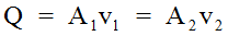
Equation 6-1.
where:
- Anchor: #NSHQGNFS
- Q = discharge (cfs or m3/s) Anchor: #NEARAKTC
- A = flow cross-sectional area (sq. ft. or m2) Anchor: #HQDGUWWR
- v = mean cross-sectional velocity (fps or m/s, perpendicular to the flow area). Anchor: #COKRDLEC
- The superscripts 1 and 2 refer to successive cross sections along the flow path.
As indicated by the Continuity Equation, the average velocity in a channel cross-section, (v) is the total discharge divided by the cross-sectional area of flow perpendicular to the cross-section. It is only a general indicator and does not reflect the horizontal and vertical variation in velocity.
Velocity varies horizontally and vertically across a section. Velocities near the ground approach zero. Highest velocities typically occur some depth below the water surface near the station where the deepest flow exists. For one-dimensional analysis techniques such as the Slope Conveyance Method and (Standard) Step Backwater Method (see Chapter 7), ignore the vertical distribution, and estimate the horizontal velocity distribution by subdividing the channel cross section and computing average velocities for each subsection. The resulting velocities represent a velocity distribution.
Channel Capacity
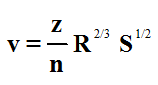
Most of the departmental channel analysis procedures use the Manning’s Equation for uniform flow (Equation 6‑2) as a basis for analysis:
Equation 6-2.
where:
- Anchor: #WGLTGNUB
- v = Velocity in cfs or m3/sec Anchor: #FCOHWIKV
- z = 1.486 for English measurement units, and 1.0 for metric Anchor: #PFXLFIPQ
- n = Manning’s roughness coefficient (a coefficient for quantifying the roughness characteristics of the channel) Anchor: #XKHTDEWO
- R = hydraulic radius (ft. or m) = A / WP Anchor: #ECQWOKKI
- WP = wetted perimeter of flow (the length of the channel boundary in direct contact with the water) (ft. or m) Anchor: #JQAIJKWT
- S = slope of the energy gradeline (ft./ft. or m/m) (For uniform, steady flow, S = channel slope, ft./ft. or m/m).
Combine Manning’s Equation with the continuity equation to determine the channel uniform flow capacity as shown in Equation 6‑3.
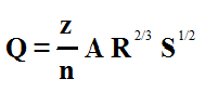
Equation 6-3.
where:
- Anchor: #IMADAFBA
- Q = discharge (cfs or m3/s) Anchor: #WGNJLFCO
- z = 1.486 for English measurement units, and 1.0 for metric Anchor: #RKIPLJIR
- A = cross-sectional area of flow (sq. ft. or m2).
For convenience, Manning’s Equation in this manual assumes the form of Equation 6‑3. Since Manning’s Equation does not allow a direct solution to water depth (given discharge, longitudinal slope, roughness characteristics, and channel dimensions), an indirect solution to channel flow is necessary. This is accomplished by developing a stage-discharge relationship for flow in the stream.
All conventional procedures for developing the stage-discharge relationship include certain basic parameters as follows:
- Anchor: #KPGWOSEK
- geometric descriptions of typical cross section Anchor: #HYRMCDAG
- identification and quantification of stream roughness characteristics Anchor: #ELJKILGN
- a longitudinal water surface slope.
You need careful consideration to make an appropriate selection and estimation of these parameters.
Anchor: #i1007491Conveyance
In channel analysis, it is often convenient to group the channel cross-sectional properties in a single term called the channel conveyance (K), shown in Equation 6‑4.
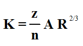
Equation 6-4.
Manning’s Equation can then be written as:
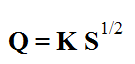
Equation 6-5.
Conveyance is useful when computing the distribution of overbank flood flows in the cross section and the flow distribution through the opening in a proposed stream crossing.
Anchor: #i1007523Energy Equations
Assuming channel slopes of less than 10 percent, the total energy head can be shown as Equation 6-6.
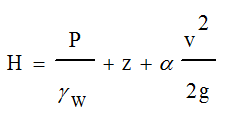
Equation 6-6.
where:
- Anchor: #OECCFPBY
- H = total energy head (ft. or m) Anchor: #VCTQQLNU
- P = pressure (lb./sq.ft. or N/m2) Anchor: #BLOGCAAT
- γw = unit weight of water (62.4 lb./cu.ft. or 9810 N/m3) Anchor: #XNGFKEPA
- z = elevation head
(ft. or m)
 = average velocity head, hv (ft.
or m)
Anchor: #CPNDMHMB
= average velocity head, hv (ft.
or m)
Anchor: #CPNDMHMB - g = gravitational acceleration (32.2 ft./ s2 or 9.81 m/s2) Anchor: #JXGLPRDH
- α = kinetic energy coefficient, as described in Kinetic Energy Coefficient Computation section Anchor: #VDUIIPKT
- v = mean velocity (fps or m/s).
In open channel computations, it is often useful to define the total energy head as the sum of the specific energy head and the elevation of the channel bottom with respect to some datum.
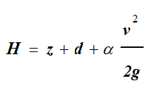
Equation 6-7.
where:
- Anchor: #YGMTJHHJ
- d = depth of flow (ft. or m).
For some applications, it may be more practical to compute the total energy head as a sum of the water surface elevation (relative to mean sea level) and velocity head.
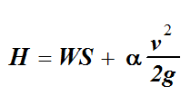
Equation 6-8.
where:
- Anchor: #IYJTNYWI
- WS = water-surface elevation or stage (ft. or m) = z + d.
Specific Energy Equation. If the channel is not too steep (slope less than 10 percent) and the streamlines are nearly straight and parallel, the specific energy, E, becomes the sum of the depth of flow and velocity head.
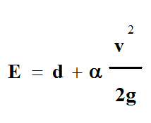
Equation 6-9.
Kinetic Energy Coefficient. Some of the numerous factors that cause variations in velocity from point to point in a cross section are channel roughness, non-uniformities in channel geometry, bends, and upstream obstructions.
The velocity head based on average velocity does not give a true measure of the kinetic energy of the flow because the velocity distribution in a river varies from a maximum in the main channel to essentially zero along the banks. Get a weighted average value of the kinetic energy by multiplying average velocity head by the kinetic energy coefficient (α). The kinetic energy coefficient is taken to have a value of 1.0 for turbulent flow in prismatic channels (channels of constant cross section, roughness, and slope) but may be significantly different than 1.0 in natural channels. Compute the kinetic energy coefficient with Equation 6‑10:
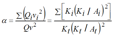
Equation 6-10.
where:
- Anchor: #BVCUFOSI
- vi = average velocity in subsection (ft./s or m/s) (see Continuity Equation section) Anchor: #NUKJATXT
- Qi = discharge in same subsection (cfs or m3/s) (see Continuity Equation section) Anchor: #QQPGFLVU
- Q = total discharge in channel (cfs or m3/s) Anchor: #WHCHFBDI
- v = average velocity in river at section or Q/A (ft./s or m/s) Anchor: #YHXXVUAL
- Ki = conveyance in subsection (cfs or m3/s) (see Conveyance section) Anchor: #YBVOFCVJ
- Ai = flow area of same subsection (sq. ft. or m2) Anchor: #QNQUYLKV
- Kt = total conveyance for cross-section (cfs or m3/s) Anchor: #YSLSEQXU
- At = total flow area of cross-section (sq. ft. or m2).
In manual computations, it is possible to account for dead water or ineffective flows in parts of a cross section by assigning values of zero or negative numbers for the subsection conveyances. The kinetic energy coefficient will, therefore, be properly computed. In computer models, however, it is not easy to assign zero or negative values because of the implicit understanding that conveyance and discharge are similarly distributed across a cross section. This understanding is particularly important at bends, embankments, and expansions, and at cross sections downstream from natural and manmade constrictions. The subdivisions should isolate any places where ineffective or upstream flow is suspected. Then, by omitting the subsections or assigning very large roughness coefficients to them, a more realistic kinetic energy coefficient is computed.
In some cases, your calculations may show kinetic energy coefficients in excess of 20, with no satisfactory explanations for the enormous magnitude of the coefficient. If adjacent cross sections have comparable values or if the changes are not sudden between cross sections, such values can be accepted. If the change is sudden, however, make some attempt to attain uniformity, such as using more cross sections to achieve gradual change, or by re-subdividing the cross section.
Energy Balance Equation
The Energy Balance Equation, Equation 6‑1, relates the total energy of an upstream section (2) along a channel with the total energy of a downstream section (1). The parameters in the Energy Equation are illustrated in Figure 6‑1. Equation 6-1 now can be expanded into Equation 6-11:
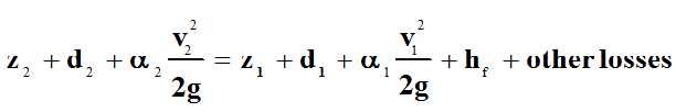
Equation 6-11.
where:
- Anchor: #CCKSJMTQ
- z = elevation of the streambed (ft. or m) Anchor: #ACUPPEVL
- d = depth of flow (ft. or m) Anchor: #KYMGGFKQ
- α = kinetic energy coefficient Anchor: #WBDCUXOE
- v = average velocity of flow (fps or m/s) Anchor: #UUSRVFAR
- hf = friction head loss from upstream to downstream (ft. or m) Anchor: #PQIGKYBT
- g = acceleration due to gravity = 32.2 ft/ s2 or 9.81 m/s2.
The energy grade line (EGL) is the line that joins the elevations of the energy head associated with a water surface profile (see Figure 6‑1).
")
Figure 6-1. EGL for Water Surface Profile
Depth of Flow
Uniform depth (du) of flow (sometimes referred to as normal depth of flow) occurs when there is uniform flow in a channel or conduit. Uniform depth occurs when the discharge, slope, cross-sectional geometry, and roughness characteristics are constant through a reach of stream. See Slope Conveyance Method for how to determine uniform depth of flow in an open channel (Chapter 7).
By plotting specific energy against depth of flow for constant discharge, a specific energy diagram is obtained (see Figure 6‑2). When specific energy is a minimum, the corresponding depth is critical depth (dc). Critical depth of flow is a function of discharge and channel geometry. For a given discharge and simple cross-sectional shapes, only one critical depth exists. However, in a compound channel such as a natural floodplain, more than one critical depth may exist.
")
Figure 6-2. Typical Specific Energy Diagram
You can calculate critical depth in rectangular channels with the following Equation 6‑12:
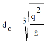
Equation 6-12.
where:
- Anchor: #EKCOVIHD
- q = discharge per ft. (m) of width (cfs/ft. or m3/s/m).
You can determine the critical depth for a given discharge and cross section iteratively with Equation 6‑13:
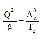
Equation 6-13.
where:
- Anchor: #TJDQSMIN
- Tc = water surface width for critical flow (ft. or m) Anchor: #SSQTQCFU
- Ac = area for critical flow (sq. ft. or m2).
Froude Number
The Froude Number (Fr) represents the ratio of inertial forces to gravitational forces and is calculated using Equation 6‑14.
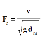
Equation 6-14.
where:
- Anchor: #NBNSOHVF
- v = mean velocity (fps or m/s) Anchor: #OPLGTIOS
- g = acceleration of gravity (32.2 ft/ s2 or 9.81 m/s2) Anchor: #DXWYLPII
- dm = hydraulic mean depth = A / T (ft. or m) Anchor: #JYAUBCWL
- A = cross-sectional area of flow (sq. ft. or m2) Anchor: #KPTJDWII
- T = channel top width at the water surface (ft. or m).
The expression for the Froude Number applies to any single section of channel. The Froude Number at critical depth is always 1.0.
Flow Types
Several recognized types of flow are theoretically possible in open channels. The methods of analysis as well as certain necessary assumptions depend on the type of flow under study. Open channel flow is usually classified as uniform or non-uniform, steady or unsteady, or or critical or supercritical.
Non-uniform, unsteady, subcritical flow is the most common type of flow in open channels in Texas. Due to the complexity and difficulty involved in the analysis of non-uniform, unsteady flow, most hydraulic computations are made with certain simplifying assumptions which allow the application of steady, uniform, or gradually varied flow principles and one-dimensional methods of analysis.
Steady, Uniform Flow. Steady flow implies that the discharge at a point does not change with time, and uniform flow requires no change in the magnitude or direction of velocity with distance along a streamline such that the depth of flow does not change with distance along a channel. Steady, uniform flow is an idealized concept of open channel flow that seldom occurs in natural channels and is difficult to obtain even in model channels. However, for practical highway applications, the flow is steady, and changes in width, depth, or direction (resulting in non-uniform flow) are sufficiently small so that flow can be considered uniform. A further assumption of rigid, uniform boundary conditions is necessary to satisfy the conditions of constant flow depth along the channel. Alluvial, sand bed channels do not exhibit rigid boundary characteristics.
Steady, Non-uniform Flow. Changes in channel characteristics often occur over a long distance so that the flow is non-uniform and gradually varied. Consideration of such flow conditions is usually reasonable for calculation of water surface profiles in Texas streams, especially for the hydraulic design of bridges.
Subcritical/Supercritical Flow. Most Texas streams flow in what is regarded as a subcritical flow regime. Subcritical flow occurs when the actual flow depth is higher than critical depth. A Froude Number less than 1.0 indicates subcritical flow. This type of flow is tranquil and slow and implies flow control from the downstream direction. Therefore, the analysis calculations are carried out from downstream to upstream. In contrast, supercritical flow is often characterized as rapid or shooting, with flow depths less than critical depth. A Froude Number greater than 1.0 indicates supercritical flow. The location of control sections and the method of analysis depend on which type of flow prevails within the channel reach under study. A Froude number equal to, or close to, 1.0 indicates instability in the channel or model. A Froude number of 1.0 should be avoided if at all possible.
Anchor: #i1007971Cross Sections
A typical cross section represents the geometric and roughness characteristics of the stream reach in question. Figure 6‑3 is an example of a plotted cross section.
")
Figure 6-3. Plotted Cross Section
Most of the cross sections selected for determining the water surface elevation at a highway crossing should be downstream of the highway because most Texas streams exhibit subcritical flow. Calculate the water surface profile through the cross sections from downstream to upstream. Generate enough cross sections upstream to determine properly the extent of the backwater created by the highway crossing structure. See Chapter 4 for details on cross sections.
Anchor: #i1007997Roughness Coefficients
All water channels, from natural stream beds to lined artificial channels, exhibit some resistance to water flow, and that resistance is referred to as roughness. Hydraulic roughness is not necessarily synonymous with physical roughness. All hydraulic conveyance formulas quantify roughness subjectively with a coefficient. In Manning’s Equation, the roughness coefficients, or n-values, for Texas streams and channels range from 0.200 to 0.012; values outside of this range are probably not realistic.
Determination of a proper n-value is the most difficult and critical of the engineering judgments required when using the Manning’s Equation.
You can find suggested values for Manning’s roughness coefficient (“n” values) in design charts such as the one shown in the file named nvalues.doc ( NVALUES). Any convenient, published design guide can be referenced for these values. Usually, reference to more than one guide can be productive in that more opinions are collected. You can find a productive and systematic approach for this task in the FHWA publication TS-84-204, Guide for Selecting Manning’s Roughness Coefficients for Natural Channels and Flood Plains.
However inexact and subjective the n-value determination may be, the n-values in a cross section are definite and unchangeable for a particular discharge and flow depth. Therefore, once you have carefully chosen the n-values, do not adjust them just to provide another answer. If there is uncertainty about particular n-value choices, consult a more experienced designer.
In some instances, such as a trapezoidal section under a bridge, the n-value may vary drastically within a section, but you should not subdivide the section. If the n-value varies as such, use a weighted n-value (nw). This procedure is defined by Equation 6‑15 as follows:
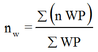
Equation 6-15.
where:
- Anchor: #RNPKKKKY
- WP = subsection wetted perimeter Anchor: #OXJCRQGI
- n = subsection n-value.
Subdividing Cross Sections
Because any estimating method involves the calculation of a series of hydraulic characteristics of the cross section, arbitrary water-surface elevations are applied to the cross section. The computation of flow or conveyance for each water-surface application requires a hydraulic radius, as seen in Figure 6‑4. The hydraulic radius is intended as an average depth of a conveyance. A hydraulic radius and subsequent conveyance is calculated under each arbitrary water surface elevation. If there is significant irregularity in the depth across the section, the hydraulic radius may not accurately represent the flow conditions. Divide the cross section into sufficient subsections so that realistic hydraulic radii are derived.
")
Figure 6-4. Cross Section Area and Wetted Perimeter
Subsections may be described with boundaries at changes in geometric characteristics and changes in roughness elements (see Figure 6‑5). Note that the vertical length between adjacent subsections is not included in the wetted perimeter. The wetted perimeter is considered only along the solid boundaries of the cross sections, not along the water interfaces between subsections.
Adjacent subsections may have identical n-values. However, the calculation of the subsection hydraulic radius will show a more consistent pattern as the tabulation of hydraulic characteristics of the cross section is developed.
")
Figure 6-5. Subdividing With Respect to Geometry and Roughness
Subdivide cross sections primarily at major breaks in geometry. Additionally, major changes in roughness may call for additional subdivisions. You need not subdivide basic shapes that are approximately rectangular, trapezoidal, semicircular, or triangular.
Subdivisions for major breaks in geometry or for major changes in roughness should maintain these approximate basic shapes so that the distribution of flow or conveyance is nearly uniform in a subsection.
Anchor: #i1008108Importance of Correct Subdivision
The importance of proper subdivision as well as the effects of improper subdivision can be illustrated dramatically. Figure 6‑6 shows a trapezoidal cross section having heavy brush and trees on the banks and subdivided near the bottom of each bank because of the abrupt change of roughness.
")
Figure 6-6. Subdivision of a Trapezoidal Cross Section
The conveyance for each subarea is calculated as follows:
|
A1 = A3 = 50 ft2 |
A1 = A3 = 4.5 m2 |
|---|---|
|
P1 = P3 = 14.14 ft |
P1 = P3 = 4.24 m |
|
R1 = R3 = A1/P1 = 3.54 ft |
R1 = R3 = A1/P1 = 1.06 m |
|
K1 = K3 = 1.486A1R12/3/n = 1724.4 cfs |
K1 = K3 = A1R12/3/n = 46.8 m3/s |
|
|
|
|
A2 = 500 ft2 |
A2 = 45 m2 |
|
P2 = 50 ft |
P2 = 15 m |
|
R2 = A2/P2 = 10 ft |
R2 = A2/P2 = 3 m |
|
K2 = 1.486A2R22/3/n = 98534.3 cfs |
K2 = A2R22/3/n = 2674.4 m3/s |
When the subareas are combined, the effective n-value for the total area can be calculated.
|
Ac = A1 + A2 + A3 = 600 ft2 |
Ac = A1 + A2 + A3 = 54 m2 |
|---|---|
|
Pc = P1 + P2 + P3 = 78.28 ft |
Pc = P1 + P2 + P3 = 23.5 m |
|
Rc = Ac/Pc = 7.66 ft |
Rc = Ac/Pc = 2.3 m |
|
KT = K1 + K2 + K3 = 101983 cfs |
KT = K1 + K2 + K3 = 2768 m3/s |
|
n = 1.486AcRc2/3/KT = 0.034 |
n = AcRc2/3/KT = 0.034 |
A smaller wetted perimeter in respect to area abnormally increases the hydraulic radius (R = A / P), and this results in a computed conveyance different from that determined for a section with a complete wetted perimeter. As shown above, a conveyance (KT) for the total area would require a composite n-value of 0.034. This is less than the n-values of 0.035 and 0.10 that describe the roughness for the various parts of the basic trapezoidal shape. Do not subdivide the basic shape. Assign an effective value of n somewhat higher than 0.035 to this cross section, to account for the additional drag imposed by the larger roughness of the banks.
At the other extreme, you must subdivide the panhandle section in Figure 6‑7, consisting of a main channel and an overflow plain, into two parts. The roughness coefficient is 0.040 throughout the total cross section. The conveyance for each subarea is calculated as follows:
|
A1 = 195 ft2 |
A1 = 20 m2 |
|---|---|
|
P1 = 68 ft |
P1 = 21 m |
|
R1 = A1/P1 = 2.87 ft |
R1 = A1/P1 = 0.95 m |
|
K1 = 1.486A1R12/3/n = 14622.1 cfs |
K1 = A1R12/3/n = 484.0 m3/s |
|
|
|
|
A2 = 814.5 ft2 |
A2 = 75.5 m2 |
|
P2 = 82.5 ft |
P2 = 24.9 m |
|
R2 = A2/P2 = 9.87 ft |
R2 = A2/P2 = 3.03 m |
|
K2 = 1.486A2R22/3/n = 139226.2 cfs |
K2 = A2R22/3/n = 3954.2 m3/s |
The effective n-value calculations for the combined subareas are as follows:
|
Ac = A1 + A2 = 1009.5 ft2 |
Ac = A1 + A2 = 95.5 m2 |
|---|---|
|
Pc = P1 + P2 = 150.5 ft |
Pc = P1 + P2 = 45.9 m |
|
Rc = Ac/Pc = 6.71 ft |
Rc = Ac/Pc = 2.08 m |
|
KT = K1 + K2 = 153848.3 cfs |
KT = K1 + K2 = 4438.2 m3/s |
|
n = 1.486AcRc2/3/KT = 0.035 |
n = AcRc2/3/KT = 0.035 |
If you do not subdivide the section, the increase in wetted perimeter of the floodplain is relatively large with respect to the increase in area. The hydraulic radius is abnormally reduced, and the calculated conveyance of the entire section (Kc) is lower than the conveyance of the main channel, K2. You should subdivide irregular cross sections such as that in Figure 6‑7 to create individual basic shapes.
")
Figure 6-7. Subdividing a “Panhandle” Cross Section
The cross section shapes in Figure 6‑6 through Figure 6‑9 represent extremes of the problems associated with improper subdivision. A bench panhandle, or terrace, is a shape that falls between these two extremes (see Figure 6‑8). Subdivide bench panhandles if the ratio L/d is equal to five or greater.
")
Figure 6-8. Bench Panhandle Cross Section
The following guidelines apply to the subdivision of triangular sections (see Figure 6‑9):
- Anchor: #QKDFHDNO
- Subdivide if the central angle is 150 or more (L/d is five or greater). Anchor: #NPJESNSB
- If L/d is almost equal to five, then subdivide at a distance of L/4 from the edge of the water. Anchor: #DVAVEVTS
- Subdivide in several places if L/d is equal to or greater than 20. Anchor: #XLRYLBUL
- No subdivisions are required on the basis of shape alone for small values of L/y, but subdivisions are permissible on the basis of roughness distribution.
")
Figure 6-9. Triangular Cross Section
Figure 6‑10 shows another shape that commonly causes problems in subdivision. In this case, subdivide the cross section if the main-channel depth (dmax) is more than twice the depth at the stream edge of the overbank area (db).
")
Figure 6-10. Problematic Cross Section
In some cases the decision to subdivide is difficult. Subdivisions in adjacent sections along the stream reach should be similar to avoid large differences in the kinetic energy coefficient (α). Therefore, if a borderline case is between sections not requiring subdivision, do not subdivide the borderline section. If it is between sections that must be subdivided, subdivide this section as well.