Section 12: Rational Method
The Rational method is appropriate for estimating peak discharges for small drainage areas of up to about 200 acres (80 hectares) with no significant flood storage. The method provides the designer with a peak discharge value, but does not provide a time series of flow nor flow volume.
Anchor: #i1469973Assumptions and Limitations
Use of the rational method includes the following assumptions and limitations:
- Anchor: #REKEJIFK
- The method is applicable if tc for the drainage area is less than the duration of peak rainfall intensity. Anchor: #IMJMNFHI
- The calculated runoff is directly proportional to the rainfall intensity. Anchor: #KMLFEMKG
- Rainfall intensity is uniform throughout the duration of the storm. Anchor: #LEKFFMKI
- The frequency of occurrence for the peak discharge is the same as the frequency of the rainfall producing that event. Anchor: #KSJMMIMN
- Rainfall is distributed uniformly over the drainage area. Anchor: #JNKGHMFK
- The minimum duration to be used for computation of rainfall intensity is 10 minutes. If the time of concentration computed for the drainage area is less than 10 minutes, then 10 minutes should be adopted for rainfall intensity computations. Anchor: #PEKFMHFF
- The rational method does not account for storage in the drainage area. Available storage is assumed to be filled.
The above assumptions and limitations are the reason the rational method is limited to watersheds 200 acres or smaller. If any one of these conditions is not true for the watershed of interest, the designer should use an alternative method.
The rational method represents a steady inflow-outflow condition of the watershed during the peak intensity of the design storm. Any storage features having sufficient volume that they do not completely fill and reach a steady inflow-outflow condition during the duration of the design storm cannot be properly represented with the rational method. Such features include detention ponds, channels with significant volume, and floodplain storage. When these features are present, an alternate rainfall-runoff method is required that accounts for the time-varying nature of the design storm and/or filling/emptying of floodplain storage. In these cases, the hydrograph method is recommended.
The steps in developing and applying the rational method are illustrated in Figure 4-8.
")
Figure 4-8. Steps in developing and applying the rational method
Anchor: #i1154472Procedure for using the Rational Method
The rational formula estimates the peak rate of runoff at a specific location in a watershed as a function of the drainage area, runoff coefficient, and mean rainfall intensity for a duration equal to the time of concentration. The rational formula is:

Equation 4-20.
Where:
- Anchor: #EMGLIHIL
- Q = maximum rate of runoff (cfs or m3/sec.) Anchor: #JKHMKKEI
- C = runoff coefficient Anchor: #NJJFKKLN
- I = average rainfall intensity (in./hr. or mm/hr.) Anchor: #JHIKIKLJ
- A = drainage area (ac or ha) Anchor: #NVHLLKMG
- Z = conversion factor, 1 for English, 360 for metric
Rainfall Intensity
The rainfall intensity (I) is the average rainfall rate in in./hr. for a specific rainfall duration and a selected frequency. The duration is assumed to be equal to the time of concentration. For drainage areas in Texas, you may compute the rainfall intensity using Equation 4-21, which is known as a rainfall intensity-duration-frequency (IDF) relationship (power-law model).
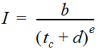
Equation 4-21.
Where:
- Anchor: #PWXYLRRI
- I = design rainfall intensity (in./hr.) Anchor: #RRWAKDYI
- tc = time of concentration (min) as discussed in Section 11 Anchor: #OMHLFKWM
- e, b, d = coefficients based on rainfall IDF data.
In September 2018, the National Oceanic and Atmospheric Administration (NOAA) released updated precipitation frequency estimates for Texas. These estimates are available through NOAA's Precipitation Frequency Data Server (PFDS) website and the report documenting the approach is also available at the same website - NOAA Atlas 14, Volume 11: Precipitation-Frequency Atlas of the United States. This new rainfall data is considered best available data and should be used for all projects. Tabular IDF data are available from the PFDS, but linear interpolation or curve generation is needed to obtain intensity values between tabular durations. Ongoing TxDOT research will produce future e, b, d coefficients to better automate intensity calculations. However, barring significant project implementation concerns, Atlas 14 IDF data should be used. Exceptions must be approved by the DHE or DES HYD and noted on the plans or drainage report.
Currently, the coefficients in Equation 4-21 can be found in the EBDLKUP-2015v2.1.xlsx spreadsheet lookup tool (developed by Cleveland et al. 2015) for specific frequencies listed by county (See video/tutorial on the use of the EBDLKUP-2015v2.1.xlsx spreadsheet tool). This spreadsheet is based on prior rainfall frequency-duration data contained in the Atlas of Depth-Duration Frequency (DDF) of Precipitation of Annual Maxima for Texas (TxDOT 5-1301-01-1).
If a project is approved to use the older values from the EBDLKUP-2015v2.1.xlsx spreadsheet lookup tool or from existing functionality in design software like GEOPAK, they should still evaluate the new NOAA rainfall changes for their project area and, if there are increases for the design frequency, estimate an appropriate level of freeboard for use. The freeboard amount and a description of how it was generated should be noted in both the plans and the drainage report. Software that facilitates Rational Method calculations often has IDF curves from rainfall data embedded into the software. Location-specific IDF from the new NOAA rainfall data can be imported for each project into the software.
TxDOT is currently working with Texas Transportation Institute (TTI) staff, as part of research project 0-6980, to update the IDF curve relationships for the state of Texas based on the 2018 NOAA rainfall data. This work will include an update of the EBDLKUP-2015v2.1.xlsx file linked above and planned for inclusion in the next HDM update.
The general shape of a rainfall IDF curve is shown in Figure 4-9. As rainfall duration approaches zero, the rainfall intensity tends towards infinity. Because the rainfall intensity/duration relationship is assessed by assuming that the duration is equal to the time of concentration, small areas with exceedingly short times of concentration could result in design rainfall intensities that are unrealistically high. To minimize this likelihood, use a minimum time of concentration of 10 minutes. As the duration tends to infinity, the design rainfall tends towards zero. Usually, the area limitation of 200 acres for Rational Method calculations should result in rainfall intensities that are not unrealistically low. However, if the estimated time of concentration is extremely long, such as may occur in extremely flat areas, it may be necessary to consider an upper threshold of time or use a different hydrologic method.
")
Figure 4-9. Typical Rainfall Intensity Duration Frequency Curve
In some instances alternate methods of determining rainfall intensity may be desired, especially for coordination with other agencies. Ensure that any alternate methods are applicable and documented.
Runoff Coefficients
Urban Watersheds
Table 4-10 suggests ranges of C values for urban watersheds for various combinations of land use and soil/surface type. This table is typical of design guides found in civil engineering texts dealing with hydrology.
|
Type of drainage area |
Runoff coefficient |
|---|---|
|
Business: |
|
|
Downtown areas |
0.70-0.95 |
|
Neighborhood areas |
0.30-0.70 |
|
Residential: |
|
|
Single-family areas |
0.30-0.50 |
|
Multi-units, detached |
0.40-0.60 |
|
Multi-units, attached |
0.60-0.75 |
|
Suburban |
0.35-0.40 |
|
Apartment dwelling areas |
0.30-0.70 |
|
Industrial: |
|
|
Light areas |
0.30-0.80 |
|
Heavy areas |
0.60-0.90 |
|
Parks, cemeteries |
0.10-0.25 |
|
Playgrounds |
0.30-0.40 |
|
Railroad yards |
0.30-0.40 |
|
Unimproved areas: |
|
|
Sand or sandy loam soil, 0-3% |
0.15-0.20 |
|
Sand or sandy loam soil, 3-5% |
0.20-0.25 |
|
Black or loessial soil, 0-3% |
0.18-0.25 |
|
Black or loessial soil, 3-5% |
0.25-0.30 |
|
Black or loessial soil, > 5% |
0.70-0.80 |
|
Deep sand area |
0.05-0.15 |
|
Steep grassed slopes |
0.70 |
|
Lawns: |
|
|
Sandy soil, flat 2% |
0.05-0.10 |
|
Sandy soil, average 2-7% |
0.10-0.15 |
|
Sandy soil, steep 7% |
0.15-0.20 |
|
Heavy soil, flat 2% |
0.13-0.17 |
|
Heavy soil, average 2-7% |
0.18-0.22 |
|
Heavy soil, steep 7% |
0.25-0.35 |
|
Streets: |
|
|
Asphaltic |
0.85-0.95 |
|
Concrete |
0.90-0.95 |
|
Brick |
0.70-0.85 |
|
Drives and walks |
0.75-0.95 |
|
Roofs |
0.75-0.95 |
Rural and Mixed-Use Watershed
Table 4-11 shows an alternate, systematic approach for developing the runoff coefficient. This table applies to rural watersheds only, addressing the watershed as a series of aspects. For each of four aspects, the designer makes a systematic assignment of a runoff coefficient “component.” Using Equation 4-22, the four assigned components are added to form an overall runoff coefficient for the specific watershed segment.
The runoff coefficient for rural watersheds is given by:
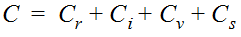
Equation 4-22.
Where:
- Anchor: #KLIKNNFE
- C = runoff coefficient for rural watershed Anchor: #FHIJKNEE
- Cr = component of coefficient accounting for watershed relief Anchor: #JNIIHMMN
- Ci = component of coefficient accounting for soil infiltration Anchor: #OLJNLNEF
- Cv = component of coefficient accounting for vegetal cover Anchor: #KLIKLLNK
- Cs = component of coefficient accounting for surface type
The designer selects the most appropriate values for Cr, Ci, Cv, and Cs from Table 4-11.
|
Watershed characteristic |
Extreme |
High |
Normal |
Low |
|---|---|---|---|---|
|
Relief - Cr |
0.28-0.35 Steep, rugged terrain with average slopes above 30% |
0.20-0.28 Hilly, with average slopes of 10-30% |
0.14-0.20 Rolling, with average slopes of 5-10% |
0.08-0.14 Relatively flat land, with average slopes of 0-5% |
|
Soil infiltration - Ci |
0.12-0.16 No effective soil cover; either rock or thin soil mantle of negligible infiltration capacity |
0.08-0.12 Slow to take up water, clay or shallow loam soils of low infiltration capacity or poorly drained |
0.06-0.08 Normal; well drained light or medium textured soils, sandy loams |
0.04-0.06 Deep sand or other soil that takes up water readily; very light, well-drained soils |
|
Vegetal cover - Cv |
0.12-0.16 No effective plant cover, bare or very sparse cover |
0.08-0.12 Poor to fair; clean cultivation, crops or poor natural cover, less than 20% of drainage area has good cover |
0.06-0.08 Fair to good; about 50% of area in good grassland or woodland, not more than 50% of area in cultivated crops |
0.04-0.06 Good to excellent; about 90% of drainage area in good grassland, woodland, or equivalent cover |
|
Surface Storage - Cs |
0.10-0.12 Negligible; surface depressions few and shallow, drainageways steep and small, no marshes |
0.08-0.10 Well-defined system of small drainageways, no ponds or marshes |
0.06-0.08 Normal; considerable surface depression, e.g., storage lakes and ponds and marshes |
0.04-0.06 Much surface storage, drainage system not sharply defined; large floodplain storage, large number of ponds or marshes |
|
Table 4-11 note: The total runoff coefficient based on the 4 runoff components is C = Cr + Ci + Cv + Cs |
||||
While this approach was developed for application to rural watersheds, it can be used as a check against mixed-use runoff coefficients computed using other methods. In so doing, the designer would use judgment, primarily in specifying Cs, to account for partially developed conditions within the watershed.
Anchor: #IJGHMNLNMixed Land Use
For areas with a mixture of land uses, a composite runoff coefficient should be used. The composite runoff coefficient is weighted based on the area of each respective land use and can be calculated as:
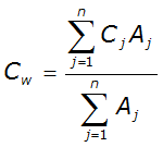
Equation 4-23.
Where:
- Anchor: #JNPIFEFK
- CW = weighted runoff coefficient Anchor: #KITIGHFL
- Cj = runoff coefficient for area j Anchor: #KONIHKFM
- Aj = area for land cover j (ft2) Anchor: #MOMGNHMK
- n = number of distinct land uses